텐서플로로 단순회귀분석 해보기 : Simple Linear Regression with Synthetic Data

텐서플로로 단순회귀분석 해보기 : Simple Linear Regression with Synthetic Data

2022. 12. 4. 15:24ㆍIT/AI

728x90

통계학에서의 단순회귀분석을 텐서플로로 해보도록 하겠습니다. 이게 일단 제일 기초죠. 꼼꼼히 살펴보시고 많은 도움이 되시기를 바랍니다.

Learning objectives:

이 연습을 수행한 후에는 다음을 수행하는 방법을 알게 됩니다.

Run Colabs.
다음 하이퍼 파라미터를 조정합니다.
학습률
시대의 수
배치 크기
다양한 종류의 손실 곡선(loss curves)을 해석합니다.

Import relevant modules

다음 셀은 프로그램에 필요한 패키지를 가져옵니다.

import pandas as pd
import tensorflow as tf
from matplotlib import pyplot as plt

Define functions that build and train a model

다음 코드는 두 가지 기능을 정의합니다. 이대로 실행해 보면 됩니다.

build_model(my_learning_rate) - 빈 모델을 빌드합니다.

#@title Define the functions that build and train a model

def build_model(my_learning_rate):

"""Create and compile a simple linear regression model."""

# Most simple tf.keras models are sequential.

# A sequential model contains one or more layers.

model = tf.keras.models.Sequential()

# Describe the topography of the model.

# The topography of a simple linear regression model

# is a single node in a single layer.

model.add(tf.keras.layers.Dense(units=1, input_shape=(1,)))

# Compile the model topography into code that

# TensorFlow can efficiently execute. Configure

# training to minimize the model's mean squared error.

model.compile(optimizer=tf.keras.optimizers.RMSprop(lr=my_learning_rate),

loss="mean_squared_error",

metrics=[tf.keras.metrics.RootMeanSquaredError()])

return model

train_model(모델, 피쳐, 레이블, 에포크) - 전달한 예제(레이블 및 레이블)에서 모델을 교육합니다.

def train_model(model, feature, label, epochs, batch_size):

"""Train the model by feeding it data."""

# Feed the feature values and the label values to the

# model. The model will train for the specified number

# of epochs, gradually learning how the feature values

# relate to the label values.

history = model.fit(x=feature,

y=label,

batch_size=batch_size,

epochs=epochs)

# Gather the trained model's weight and bias.

trained_weight = model.get_weights()[0]

trained_bias = model.get_weights()[1]

# The list of epochs is stored separately from the

# rest of history.

epochs = history.epoch

# Gather the history (a snapshot) of each epoch.

hist = pd.DataFrame(history.history)

# Specifically gather the model's root mean

# squared error at each epoch.

rmse = hist["root_mean_squared_error"]

return trained_weight, trained_bias, epochs, rmse

print("Defined build_model and train_model")

Define plotting functions

다음 두개의 그래프를 출력해주는 함수를 생성해 놓습니다.

1) 형상 값 대 레이블 값의 그림 및 훈련된 모형의 출력을 보여주는 선.

#@title Define the plotting functions

def plot_the_model(trained_weight, trained_bias, feature, label):

"""Plot the trained model against the training feature and label."""

# Label the axes.

plt.xlabel("feature")

plt.ylabel("label")

# Plot the feature values vs. label values.

plt.scatter(feature, label)

# Create a red line representing the model. The red line starts

# at coordinates (x0, y0) and ends at coordinates (x1, y1).

x0 = 0

y0 = trained_bias

x1 = feature[-1]

y1 = trained_bias + (trained_weight * x1)

plt.plot([x0, x1], [y0, y1], c='r')

# Render the scatter plot and the red line.

plt.show()

2) 손실 곡선

def plot_the_loss_curve(epochs, rmse):

"""Plot the loss curve, which shows loss vs. epoch."""

plt.figure()

plt.xlabel("Epoch")

plt.ylabel("Root Mean Squared Error")

plt.plot(epochs, rmse, label="Loss")

plt.legend()

plt.ylim([rmse.min()*0.97, rmse.max()])

plt.show()

print("Defined the plot_the_model and plot_the_loss_curve functions.")

Define the dataset

데이터 세트는 12개의 예로 구성합니다. 각 예제는 하나의 피쳐와 하나의 레이블로 구성됩니다.

my_feature = ([1.0, 2.0,  3.0,  4.0,  5.0,  6.0,  7.0,  8.0,  9.0, 10.0, 11.0, 12.0])
my_label   = ([5.0, 8.8,  9.6, 14.2, 18.8, 19.5, 21.4, 26.8, 28.9, 32.0, 33.8, 38.2])

Specify the hyperparameters

이제 하이퍼 파라미터를 조정하면서 학습률, 반복회수,배치 크기의 역할을 알아봅니다.

다음 코드 셀은 이러한 하이퍼 파라미터를 초기화한 다음 모델을 빌드하고 훈련하는 함수를 호출합니다.

학습률=0.01
반복회수=10회
배치_크기=12

learning_rate=0.01
epochs=10
my_batch_size=12

my_model = build_model(learning_rate)
trained_weight, trained_bias, epochs, rmse = train_model(my_model, my_feature, 
                                                         my_label, epochs,
                                                         my_batch_size)
plot_the_model(trained_weight, trained_bias, my_feature, my_label)
plot_the_loss_curve(epochs, rmse)

/usr/local/lib/python3.8/dist-packages/numpy/core/shape_base.py:65: VisibleDeprecationWarning: Creating an ndarray from ragged nested sequences (which is a list-or-tuple of lists-or-tuples-or ndarrays with different lengths or shapes) is deprecated. If you meant to do this, you must specify 'dtype=object' when creating the ndarray.
  ary = asanyarray(ary)

Epoch 1/10
1/1 [==============================] - 1s 562ms/step - loss: 767.2870 - root_mean_squared_error: 27.6999
Epoch 2/10
1/1 [==============================] - 0s 11ms/step - loss: 752.9022 - root_mean_squared_error: 27.4391
Epoch 3/10
1/1 [==============================] - 0s 10ms/step - loss: 742.5979 - root_mean_squared_error: 27.2507
Epoch 4/10
1/1 [==============================] - 0s 10ms/step - loss: 734.0480 - root_mean_squared_error: 27.0933
Epoch 5/10
1/1 [==============================] - 0s 13ms/step - loss: 726.5150 - root_mean_squared_error: 26.9539
Epoch 6/10
1/1 [==============================] - 0s 14ms/step - loss: 719.6575 - root_mean_squared_error: 26.8264
Epoch 7/10
1/1 [==============================] - 0s 10ms/step - loss: 713.2852 - root_mean_squared_error: 26.7074
Epoch 8/10
1/1 [==============================] - 0s 11ms/step - loss: 707.2801 - root_mean_squared_error: 26.5947
Epoch 9/10
1/1 [==============================] - 0s 11ms/step - loss: 701.5629 - root_mean_squared_error: 26.4870
Epoch 10/10
1/1 [==============================] - 0s 8ms/step - loss: 696.0779 - root_mean_squared_error: 26.3833

Examine the graphs

맨 위 그래프를 검사합니다. 파란색 점은 실제 데이터를 나타내고 빨간색 선은 훈련된 모델의 출력을 나타냅니다. 이상적으로는 빨간색 선이 파란색 점과 잘 맞아야 합니다. 그래요? 아마 아닐 것입니다.

어느 정도의 무작위성은 모델을 훈련시키는 데 사용되므로 훈련할 때마다 다소 다른 결과를 얻을 수 있습니다. 그렇기는 하지만, 여러분이 매우 운이 좋은 사람이 아니라면, 빨간 선은 아마도 파란 점들과 잘 맞지 않을 것입니다.

손실 곡선을 보여주는 아래쪽 그래프를 조사합니다. 손실 곡선은 감소하지만 평평해지지는 않습니다. 이는 모형이 충분히 훈련되지 않았음을 나타냅니다.

손실 곡선을 조사합니다. 모델이 수렴됩니까?

Increase the learning rate

과제 2에서는 모형을 수렴하기 위해 에포크 수를 늘렸습니다. 때로는 학습률을 높임으로써 모델이 더 빨리 수렴되도록 할 수 있다. 그러나 학습률을 너무 높게 설정하면 모델이 수렴하는 것이 불가능한 경우가 많다. 과제 3에서는 학습률을 의도적으로 너무 높게 설정했습니다. 다음 코드 셀을 실행하여 어떤 일이 일어나는지 확인합니다.

>> 학습률을 100,반복회수도 500으로 올려보겠습니다.

# Increase the learning rate and decrease the number of epochs.
learning_rate=100 
epochs=500 

my_model = build_model(learning_rate)
trained_weight, trained_bias, epochs, rmse = train_model(my_model, my_feature, 
                                                         my_label, epochs,
                                                         my_batch_size)
plot_the_model(trained_weight, trained_bias, my_feature, my_label)
plot_the_loss_curve(epochs, rmse)

/usr/local/lib/python3.8/dist-packages/keras/optimizers/optimizer_v2/rmsprop.py:135: UserWarning: The `lr` argument is deprecated, use `learning_rate` instead.
  super(RMSprop, self).__init__(name, **kwargs)

1/1 [==============================] - 0s 307ms/step - loss: 235.4772 - root_mean_squared_error: 15.3453
Epoch 2/500
1/1 [==============================] - 0s 9ms/step - loss: 6736925.5000 - root_mean_squared_error: 2595.5588
Epoch 3/500
1/1 [==============================] - 0s 8ms/step - loss: 234.2189 - root_mean_squared_error: 15.3042
Epoch 4/500
1/1 [==============================] - 0s 10ms/step - loss: 1.7449 - root_mean_squared_error: 1.3209
Epoch 5/500
1/1 [==============================] - 0s 12ms/step - loss: 0.9076 - root_mean_squared_error: 0.9527
Epoch 6/500
1/1 [==============================] - 0s 10ms/step - loss: 0.8950 - root_mean_squared_error: 0.9461
Epoch 7/500
1/1 [==============================] - 0s 14ms/step - loss: 0.8934 - root_mean_squared_error: 0.9452
Epoch 8/500
1/1 [==============================] - 0s 12ms/step - loss: 0.8922 - root_mean_squared_error: 0.9445
Epoch 9/500
1/1 [==============================] - 0s 10ms/step - loss: 0.8910 - root_mean_squared_error: 0.9439
Epoch 10/500
1/1 [==============================] - 0s 8ms/step - loss: 0.8898 - root_mean_squared_error: 0.9433
Epoch 11/500
1/1 [==============================] - 0s 15ms/step - loss: 0.8886 - root_mean_squared_error: 0.9427
Epoch 12/500
1/1 [==============================] - 0s 12ms/step - loss: 0.8875 - root_mean_squared_error: 0.9421
Epoch 13/500
1/1 [==============================] - 0s 8ms/step - loss: 0.8864 - root_mean_squared_error: 0.9415


:
:

Epoch 497/500
1/1 [==============================] - 0s 13ms/step - loss: 170417.5312 - root_mean_squared_error: 412.8166
Epoch 498/500
1/1 [==============================] - 0s 11ms/step - loss: 170417.6406 - root_mean_squared_error: 412.8167
Epoch 499/500
1/1 [==============================] - 0s 14ms/step - loss: 170417.6719 - root_mean_squared_error: 412.8167
Epoch 500/500
1/1 [==============================] - 0s 13ms/step - loss: 170417.6406 - root_mean_squared_error: 412.8167
/usr/local/lib/python3.8/dist-packages/numpy/core/shape_base.py:65: VisibleDeprecationWarning: Creating an ndarray from ragged nested sequences (which is a list-or-tuple of lists-or-tuples-or ndarrays with different lengths or shapes) is deprecated. If you meant to do this, you must specify 'dtype=object' when creating the ndarray.
  ary = asanyarray(ary)

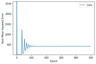
결과 모델은 끔찍합니다. 빨간색 선이 파란색 점과 일치하지 않습니다. 게다가, 손실 곡선은 롤러코스터처럼 진동한다. 진동 손실 곡선은 학습 속도가 너무 높다는 것을 강하게 시사합니다.

Find the ideal combination of epochs and learning rate

다음 두 가지 하이퍼 파라미터에 값을 할당하여 교육이 최대한 효율적으로 수렴되도록 합니다.

학습률(learning_rate)
epochs

아래 물음표를 바꾸어가면서 실행해보세요.

# Set the learning rate and number of epochs
learning_rate= ?  # Replace ? with a floating-point number
epochs= ?   # Replace ? with an integer

my_model = build_model(learning_rate)
trained_weight, trained_bias, epochs, rmse = train_model(my_model, my_feature, 
                                                         my_label, epochs,
                                                         my_batch_size)
plot_the_model(trained_weight, trained_bias, my_feature, my_label)
plot_the_loss_curve(epochs, rmse)

Adjust the batch size [ 배치사이즈의 조정 ]

시스템은 모델의 손실 값을 다시 계산하고 각 반복 후 모델의 가중치와 편향을 조정합니다. 각 반복은 시스템이 한 배치를 처리하는 범위입니다. 예를 들어 배치 크기가 6이면 시스템은 모형의 손실 값을 다시 계산하고 6개의 예제마다 처리한 후 모형의 가중치와 치우침을 조정합니다.

하나의 에포크는 데이터 세트의 모든 예제를 처리하기에 충분한 반복에 걸쳐 있다. 예를 들어 배치 크기가 12인 경우 각 에포크는 한 번의 반복을 수행합니다. 그러나 배치 크기가 6이면 각 에포크는 두 번의 반복을 소비합니다.

배치 크기를 단순히 데이터 세트의 예제 수(이 경우 12)로 설정하는 것은 유혹적이다. 그러나 모델은 실제로 소규모 배치에서 더 빠르게 훈련할 수 있습니다. 반대로, 매우 작은 배치는 모델이 수렴하는 데 도움이 되는 충분한 정보를 포함하지 않을 수 있습니다.

다음 코드 셀에서 batch_size로 실험해 보십시오. batch_size에 대해 설정할 수 있는 가장 작은 정수는 무엇이며 모델은 100개의 에포크로 수렴할 수 있습니까?

[ ]

learning_rate=0.05

epochs=100

my_batch_size= ? # Replace ? with an integer.

my_model = build_model(learning_rate)

trained_weight, trained_bias, epochs, rmse = train_model(my_model, my_feature,

my_label, epochs,

my_batch_size)

plot_the_model(trained_weight, trained_bias, my_feature, my_label)

plot_the_loss_curve(epochs, rmse)

/usr/local/lib/python3.8/dist-packages/keras/optimizers/optimizer_v2/rmsprop.py:135: UserWarning: The `lr` argument is deprecated, use `learning_rate` instead.
  super(RMSprop, self).__init__(name, **kwargs)

1/1 [==============================] - 0s 369ms/step - loss: 385.8926 - root_mean_squared_error: 19.6441
Epoch 2/100
1/1 [==============================] - 0s 11ms/step - loss: 336.3672 - root_mean_squared_error: 18.3403
Epoch 3/100
1/1 [==============================] - 0s 15ms/step - loss: 303.6651 - root_mean_squared_error: 17.4260
Epoch 4/100
1/1 [==============================] - 0s 12ms/step - loss: 278.1166 - root_mean_squared_error: 16.6768
Epoch 5/100
1/1 [==============================] - 0s 12ms/step - loss: 256.7425 - root_mean_squared_error: 16.0232
Epoch 6/100
1/1 [==============================] - 0s 12ms/step - loss: 238.1809 - root_mean_squared_error: 15.4331
Epoch 7/100
1/1 [==============================] - 0s 10ms/step - loss: 221.6801 - root_mean_squared_error: 14.8889
Epoch 8/100
1/1 [==============================] - 0s 12ms/step - loss: 206.7758 - root_mean_squared_error: 14.3797
Epoch 9/100
1/1 [==============================] - 0s 13ms/step - loss: 193.1588 - root_mean_squared_error: 13.8982
Epoch 10/100
1/1 [==============================] - 0s 9ms/step - loss: 180.6116 - root_mean_squared_error: 13.4392
:
:
:
Epoch 94/100
1/1 [==============================] - 0s 9ms/step - loss: 0.8788 - root_mean_squared_error: 0.9374
Epoch 95/100
1/1 [==============================] - 0s 9ms/step - loss: 0.8786 - root_mean_squared_error: 0.9373
Epoch 96/100
1/1 [==============================] - 0s 10ms/step - loss: 0.8784 - root_mean_squared_error: 0.9372
Epoch 97/100
1/1 [==============================] - 0s 15ms/step - loss: 0.8783 - root_mean_squared_error: 0.9372
Epoch 98/100
1/1 [==============================] - 0s 8ms/step - loss: 0.8781 - root_mean_squared_error: 0.9371
Epoch 99/100
1/1 [==============================] - 0s 9ms/step - loss: 0.8779 - root_mean_squared_error: 0.9370
Epoch 100/100
1/1 [==============================] - 0s 10ms/step - loss: 0.8777 - root_mean_squared_error: 0.9369

Epoch 1/100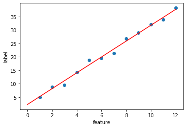

Summary of hyperparameter tuning

대부분의 기계 학습 문제는 많은 "하이퍼 파라미터" 튜닝을 필요로 한다. 안타깝게도 모든 모델에 대해 구체적인 튜닝 규칙을 제공할 수는 없습니다. 학습 속도를 낮추면 한 모델이 효율적으로 수렴하는 데 도움이 되지만 다른 모델이 지나치게 느리게 수렴하도록 만들 수 있다. 데이터 세트에 가장 적합한 하이퍼 파라미터 세트를 찾으려면 실험을 수행해야 합니다. 그렇긴 하지만, 여기 몇 가지 경험칙이 있다.

훈련 손실은 꾸준히 감소해야 하며 처음에는 가파르게 감소한 후 곡선의 기울기가 0에 도달하거나 0에 가까워질 때까지 더 느리게 감소해야 한다.
훈련 손실이 수렴되지 않으면 더 많은 반복훈련이 되게 훈련하십시오.
교육 손실이 너무 느리게 감소하는 경우 학습 속도를 높입니다. 학습 속도를 너무 높게 설정하면 훈련 손실이 수렴되는 것을 방지할 수도 있습니다.
훈련 손실이 크게 변화하는 경우(즉, 훈련 손실이 급증하는 경우), 학습 속도를 감소시킵니다.
에포크 수나 배치 크기를 늘리면서 학습 속도를 낮추는 것은 종종 좋은 조합이다.
batch size를 매우 작은 배치 번호로 설정하면 불안정해질 수도 있습니다. 먼저 큰 배치 크기 값을 시도합니다. 그런 다음 성능 저하가 나타날 때까지 배치 크기를 줄입니다.
매우 많은 예로 구성된 실제 데이터 세트의 경우 전체 데이터 세트가 메모리에 맞지 않을 수 있다. 이러한 경우 배치가 메모리에 적합하도록 배치 크기를 줄여야 합니다.
하이퍼 파라미터의 이상적인 조합은 데이터에 의존하므로 항상 실험하고 검증해야 합니다.

단순회귀분석을 해보면서 조정이 필요한 파라미터에 대해서 알아보았습니다.

그리고 또한 단순회귀분석의 코드모델도 알아보았습니다.

더욱 발전이 있으시길 바랍니다.